Geographic Analysis with R: GeoTIFF Conversion & NDVI CSV Processing

Geographic Analysis with R:
GeoTIFF Conversion & NDVI CSV Processing

Luhansk NDVI Distribution Compared Years

Developed R code with documentation

NDVI LuhanskaJune 27, 2020

NDVI LuhanskaJune 27, 2021

NDVI LuhanskaJuly 7, 2022

NDVI LuhanskaJuly 27, 2023

NDVI LuhanskaJuly 27, 2024

1. Introduction - code overview

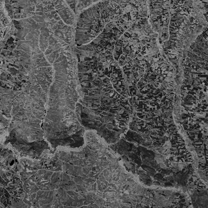
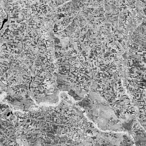
This web application provides a comprehensive guide and tools for Geographic Information System (GIS) analysis using R programming. It focuses on processing NDVI (Normalized Difference Vegetation Index) data derived from satellite imagery, specifically for the Luhansk region. Users can utilize the R code snippets provided to convert, process, and visualize the data. The application supports generating graphs in both colorful and black-and-white formats, making it ideal for research and academic publication.

The workflow is divided into sections, allowing users to follow step-by-step instructions for achieving their desired outputs. Depending on the user's needs, they can choose between two main workflows:

➊

Colorful Graphs Workflow: Use code from Chapters 2, 3, and 4 sequentially. This workflow generates colorful graphs suitable for digital presentations and displays. It provides a detailed step-by-step guide, displaying code in parts within Chapters 3 and 4, along with detailed documentation and descriptions for each part. This allows users to better understand and customize their workflow, though it may take more time to traverse multiple sections and combine snippets.

➋

Black-and-White Graphs Workflow: Use code from Chapters 2, 5, and 6. This workflow creates black-and-white graphs optimized for printing in academic articles. Chapters 5 and 6 provide singular, streamlined code snippets without additional explanations, making this workflow faster and more practical for most users. It avoids the need to connect multiple parts and works out-of-the-box for generating monochromatic graphs.

Note that Chapter 3, which converts GeoTIFF files into CSV files, is a necessary and shared step in both workflows. By following the appropriate steps, users can efficiently process NDVI data and generate visualizations tailored to their needs. The application provides a modular approach to cater to different presentation and publication formats.

2. Conversion of GeoTIFF Files to CSV

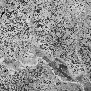
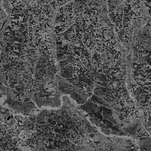
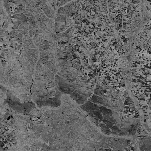
This guide demonstrates the conversion of GeoTIFF satellite imagery files into CSV format using the R programming language. The process is particularly useful for researchers working in GIS or remote sensing who need to preprocess data for statistical analysis or predictive modeling. The example uses NDVI (Normalized Difference Vegetation Index) images from the Luhansk region, extracted from QGIS.

The script utilizes the raster package in R to handle GeoTIFF files and converts them into CSV format. CSV files are more versatile for data analysis in tools such as R, Python, or machine learning models. Before running the code, ensure the raster package is installed.

➊

Check for and install the "raster" package: The script ensures that the required package is installed before proceeding.

➋

Specify input files: GeoTIFF files for NDVI images from different dates are listed.

➌

Conversion function: A function reads the raster data, converts it into a matrix, and saves it as a CSV file.

➍

Batch processing: The function is applied to multiple files to automate the conversion process.

The output files will be saved in the same directory as the input GeoTIFF files, with the .csv extension replacing .tif. This workflow simplifies data preprocessing for further spatial-temporal analysis or predictive modeling.

if (!requireNamespace("raster", quietly = TRUE)) { 
  install.packages("raster")
}
library(raster)
files <- c(
  "C:/GIS/NDVILuhanska20200627.tif",
  "C:/GIS/NDVILuhanska20210627.tif",
  "C:/GIS/NDVILuhanska20220707.tif",
  "C:/GIS/NDVILuhanska20230727.tif",
  "C:/GIS/NDVILuhanska20240727.tif"
)
tiff_to_csv <- function(file) {  
  raster_data <- raster(file)
  matrix_data <- as.matrix(raster_data)
  output_csv <- sub(".tif", ".csv", file)  
  output_csv <- sub("C:/GIS/", "C:/GIS/", output_csv)   
  write.csv(matrix_data, output_csv, row.names = FALSE)  
  return(output_csv)
}
csv_files <- lapply(files, tiff_to_csv)

3. Using RStudio to generate separate graphs for each year

3.1 NDVI Data Import – Processing of CSV Files

The first step in analyzing NDVI data involves preparing your R environment and loading the necessary libraries. This snippet ensures the required packages, dplyr and ggplot2, are installed and loaded. These libraries are essential for data manipulation and visualization tasks.

The snippet also defines the list of CSV file paths, corresponding to the NDVI data from different dates, and specifies an output directory where processed results will be saved. Each file contains numerical NDVI values for the Luhansk region that are used in subsequent steps for analysis and visualization.

if (!requireNamespace("dplyr", quietly = TRUE)) {
    install.packages("dplyr")
}
if (!requireNamespace("ggplot2", quietly = TRUE)) {
    install.packages("ggplot2")
}
library(dplyr)
library(ggplot2)

file_paths <- list(
    "C:/GIS/NDVILuhanska20200627.csv",
    "C:/GIS/NDVILuhanska20210627.csv",
    "C:/GIS/NDVILuhanska20220707.csv",
    "C:/GIS/NDVILuhanska20230727.csv",
    "C:/GIS/NDVILuhanska20240727.csv"
)

output_directory <- "C:/GIS"

3.2 Data Transformation – Preparing NDVI Data for Analysis

This snippet defines the process_file function, which processes individual CSV files containing NDVI values. The function performs the following steps:

➊

File name extraction and date formatting: Extracts the date from the file name and formats it for use in visualizations and results.

➋

Data reading and cleaning: Reads NDVI values from the CSV file and removes invalid or missing values.

➌

Grouping and summarization: Groups NDVI values into predefined ranges and calculates summary statistics, including the count of pixels, area in square meters, and scaled value averages.

➍

Output generation: Saves the summarized data to a new CSV file for further analysis or visualization.

The process_file function is applied to all CSV files, automating the data transformation process and ensuring consistency across the dataset.

process_file <- function(file_path, output_directory) {
    file_name <- tools::file_path_sans_ext(basename(file_path))
    date_part <- gsub("NDVILuhanska", "", file_name)
    date_formatted <- paste(substr(date_part, 7, 8), substr(date_part, 5, 6), substr(date_part, 1, 4), sep = "-")

    ndvi_data <- tryCatch({
        read.csv(file_path, header = FALSE)
    }, error = function(e) {
        stop(paste("Failed to load the CSV file:", file_path))
    })

    ndvi_values <- as.vector(as.matrix(ndvi_data))
    ndvi_values <- suppressWarnings(as.numeric(ndvi_values))
    ndvi_values <- ndvi_values[!is.na(ndvi_values)]
    ndvi_values <- cut(ndvi_values, breaks = seq(-1, 1, by = 0.01), include.lowest = TRUE, labels = FALSE)

    ndvi_df <- data.frame(
        value = ndvi_values,
        original_value = as.vector(as.matrix(ndvi_data))[seq_along(ndvi_values)],
        scaled_value = scale(as.numeric(ndvi_values)),
        sqrt_value = sqrt(abs(as.numeric(ndvi_values)))
    )

    result <- ndvi_df %>%
        group_by(value) %>%
        summarise(
            count = n(),
            area_m2 = count * 100,
            mean_scaled_value = mean(scaled_value, na.rm = TRUE),
            sum_sqrt_value = sum(sqrt_value, na.rm = TRUE)
        )

    csv_output_path <- file.path(output_directory, paste0(file_name, "_grouped_values.csv"))
    tryCatch({
        write.csv(result, csv_output_path, row.names = FALSE)
        cat("Results saved to", csv_output_path, "\n")
    }, error = function(e) {
        stop(paste("Failed to save results for:", file_name))
    })

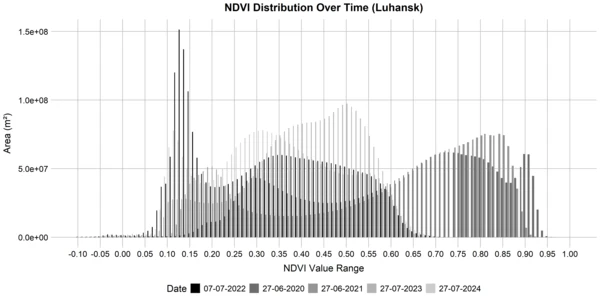
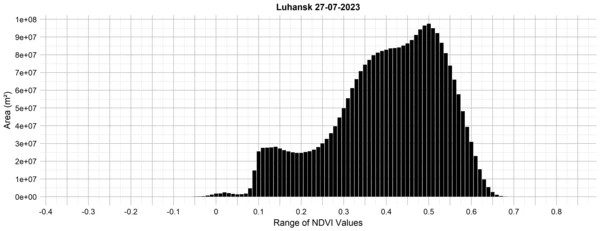
3.3 Bar Plot Generation – Visualizing NDVI Data

This section demonstrates how to generate a bar plot using the ggplot2 library in R. The bar plot represents the area (in square meters) for various NDVI value ranges. Below are the steps and details of what the code accomplishes:

➊

Data Mapping: Maps NDVI ranges to the x-axis and calculates the corresponding area (in square meters) for the y-axis.

➋

Customization: Adjusts axis labels, tick marks, grid lines, and plot title for clarity and aesthetics.

➌

Saving Output: Saves the bar plot as a PNG file in the specified output directory.

bar_plot <- ggplot(result, aes(x = as.numeric(value) * 0.01 - 1, y = area_m2)) +
        geom_bar(stat = "identity", fill = "white") +
        labs(
            title = paste("Luhansk", date_formatted),
            x = "Range of NDVI Values",
            y = "Area (m²)"
        ) +
        scale_x_continuous(
            breaks = seq(-1, 1, by = 0.05),
            labels = function(x) ifelse((seq_along(x) - 1) %% 2 == 0, x, "")
        ) +
        scale_y_continuous(breaks = scales::pretty_breaks(n = 10)) +
        theme_minimal() +
        theme(
            plot.title = element_text(color = "white", size = 12, face = "bold", hjust = 0.5, margin = margin(b = 5)),
            axis.title.x = element_text(color = "white", size = 12, margin = margin(t = 5)),
            axis.title.y = element_text(color = "white", size = 12, margin = margin(r = 5)),
            axis.text.x = element_text(color = "white", size = 12),
            axis.text.y = element_text(color = "white", size = 12),
            panel.grid.major = element_line(color = "black", size = 0.5),
            panel.grid.minor = element_line(color = "black", size = 0.2),
            panel.grid.major.x = element_line(color = ifelse(seq(-1, 1, by = 0.05) == 0, "black", "black"), size = ifelse(seq(-1, 1, by = 0.05) == 0, 1, 0.5)),
            panel.background = element_rect(fill = "transparent", color = NA),
            plot.background = element_rect(fill = "transparent", color = NA)
        )

    bar_plot_path <- file.path(output_directory, paste0(file_name, "_bar_plot.png"))
    tryCatch({
        ggsave(bar_plot_path, plot = bar_plot, width = 13, height = 5, bg = "transparent")
        cat("Bar plot saved to", bar_plot_path, "\n")
    }, error = function(e) {
        stop(paste("Failed to save bar plot for:", file_name))
    })

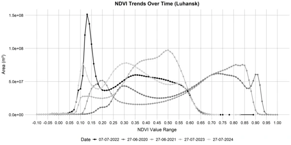
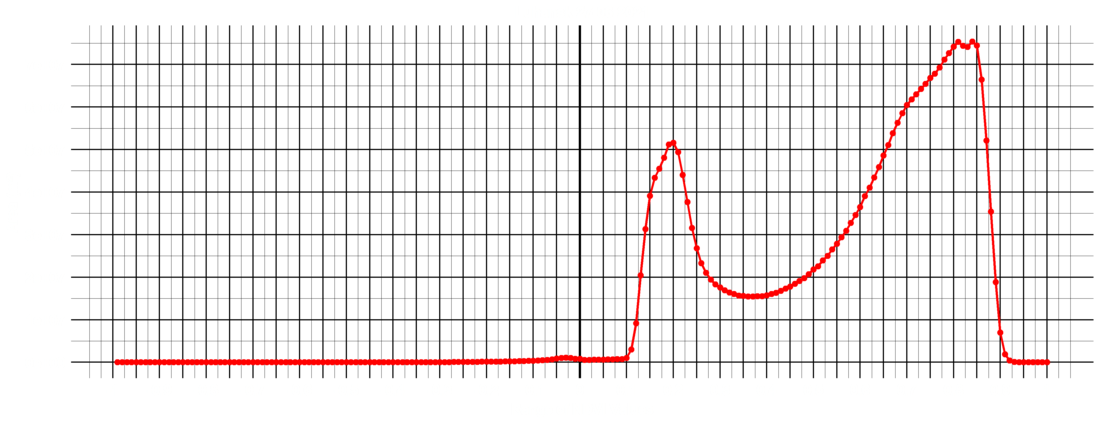
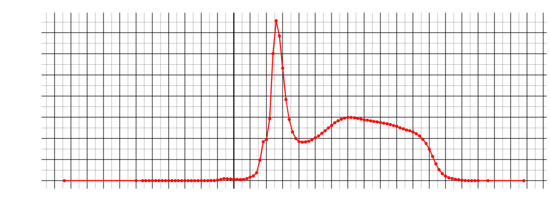
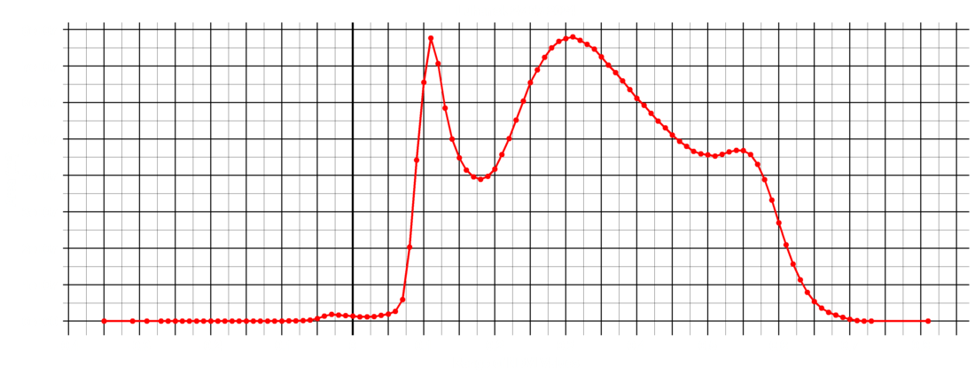
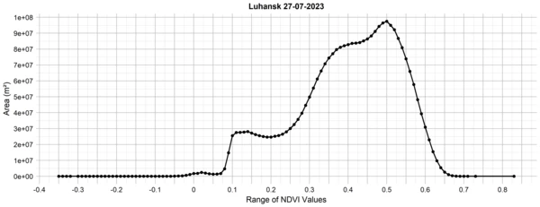
3.4 Line Plot Generation – NDVI Trends Over Ranges

This section explains how to create a line plot to visualize trends in NDVI values and their corresponding areas. Using the ggplot2 library, the code achieves the following:

➊

Line and Points: Plots NDVI ranges on the x-axis and their associated area (in square meters) on the y-axis, using a red line and point markers for emphasis.

➋

Enhanced Readability: Includes custom axis labels, grid styles, and plot titles to improve visual interpretation.

➌

Output Handling: Saves the resulting plot as a PNG file in the output directory for further use.

line_plot <- ggplot(result, aes(x = as.numeric(value) * 0.01 - 1, y = area_m2)) +
        geom_line(color = "red", size = 1) +
        geom_point(color = "red", size = 2) +
        labs(
            title = paste("Luhansk", date_formatted),
            x = "Range of NDVI Values",
            y = "Area (m²)"
        ) +
        scale_x_continuous(
            breaks = seq(-1, 1, by = 0.05),
            labels = function(x) ifelse((seq_along(x) - 1) %% 2 == 0, x, "")
        ) +
        scale_y_continuous(breaks = scales::pretty_breaks(n = 10)) +
        theme_minimal() +
        theme(
            plot.title = element_text(color = "white", size = 12, face = "bold", hjust = 0.5, margin = margin(b = 5)),
            axis.title.x = element_text(color = "white", size = 12, margin = margin(t = 5)),
            axis.title.y = element_text(color = "white", size = 12, margin = margin(r = 5)),
            axis.text.x = element_text(color = "white", size = 12),
            axis.text.y = element_text(color = "white", size = 12),
            panel.grid.major = element_line(color = "black", size = 0.5),
            panel.grid.minor = element_line(color = "black", size = 0.2),
            panel.grid.major.x = element_line(color = ifelse(seq(-1, 1, by = 0.05) == 0, "black", "black"),
             size = ifelse(seq(-1, 1, by = 0.05) == 0, 1, 0.5)),
            panel.background = element_rect(fill = "transparent", color = NA),
            plot.background = element_rect(fill = "transparent", color = NA)
        )

    line_plot_path <- file.path(output_directory, paste0(file_name, "_line_plot.png"))
    tryCatch({
        ggsave(line_plot_path, plot = line_plot, width = 13, height = 5, bg = "transparent")
        cat("Line plot saved to", line_plot_path, "\n")
    }, error = function(e) {
        stop(paste("Failed to save line plot for:", file_name))
    })

3.5 Batch Processing Completion – Finalizing Workflow

This section completes the NDVI analysis by processing multiple CSV files in a batch. The loop ensures consistency and automation across all files. Key actions performed by the code include:

➊

Iterative Processing: Iterates through a predefined list of file paths and applies the process_file function to each file.

➋

Error Handling: Includes error-catching mechanisms to handle issues such as missing files or unexpected data formats.

➌

Completion Logging: Logs the processing completion status for each file, providing a clear record of the workflow.

 cat("Processing completed for:", file_path, "\n")
}

for (file_path in file_paths) {
    process_file(file_path, output_directory)
}

4. Using RStudio to generate graphs comparing plots over the years

4.1 Setting Up Environment – Checking Packages and Preparing Data

This snippet ensures that the required packages are installed and available for use. It also defines file paths and processes the input data.

➊

Package Management: Checks if the dplyr, ggplot2, and readr libraries are installed. If not, it installs them and loads them into the R environment.

➋

File Paths Definition: Specifies the input CSV files containing NDVI data and sets the output directory for saving processed files and plots.

➌

Data Processing Loop: Iterates through each file path to:

Extract and format the date from the file name.
Read the CSV file and handle any errors gracefully.
Mutate the data to add a formatted date and NDVI range values.
Combine the processed data into a single data frame.

➍

Filtering Data: Removes rows where the NDVI range is less than -0.1 to focus on valid data.

if (!requireNamespace("dplyr", quietly = TRUE)) {
    install.packages("dplyr")
}
if (!requireNamespace("ggplot2", quietly = TRUE)) {
    install.packages("ggplot2")
}
if (!requireNamespace("readr", quietly = TRUE)) {
    install.packages("readr")
}
library(dplyr)
library(ggplot2)
library(readr)

grouped_file_paths <- list(
    "C:/GIS/NDVILuhanska20200627_grouped_values.csv",
    "C:/GIS/NDVILuhanska20210627_grouped_values.csv",
    "C:/GIS/NDVILuhanska20220707_grouped_values.csv",
    "C:/GIS/NDVILuhanska20230727_grouped_values.csv",
    "C:/GIS/NDVILuhanska20240727_grouped_values.csv"
)

output_directory <- "C:/GIS"

all_grouped_data <- data.frame()

for (file_path in grouped_file_paths) {
    file_name <- tools::file_path_sans_ext(basename(file_path))
    date_part <- gsub("NDVILuhanska", "", file_name)
    date_part <- gsub("_grouped_values", "", date_part)
    date_formatted <- paste(substr(date_part, 7, 8), substr(date_part, 5, 6), substr(date_part, 1, 4), sep = "-")

    grouped_data <- tryCatch({
        read.csv(file_path)
    }, error = function(e) {
        stop(paste("Failed to load the grouped CSV file:", file_path))
    })

    grouped_data <- grouped_data %>%
        mutate(date = date_formatted, range = as.numeric(value) * 0.01 - 1)

    all_grouped_data <- bind_rows(all_grouped_data, grouped_data)
}

all_grouped_data <- all_grouped_data %>%
    filter(range >= -0.1)

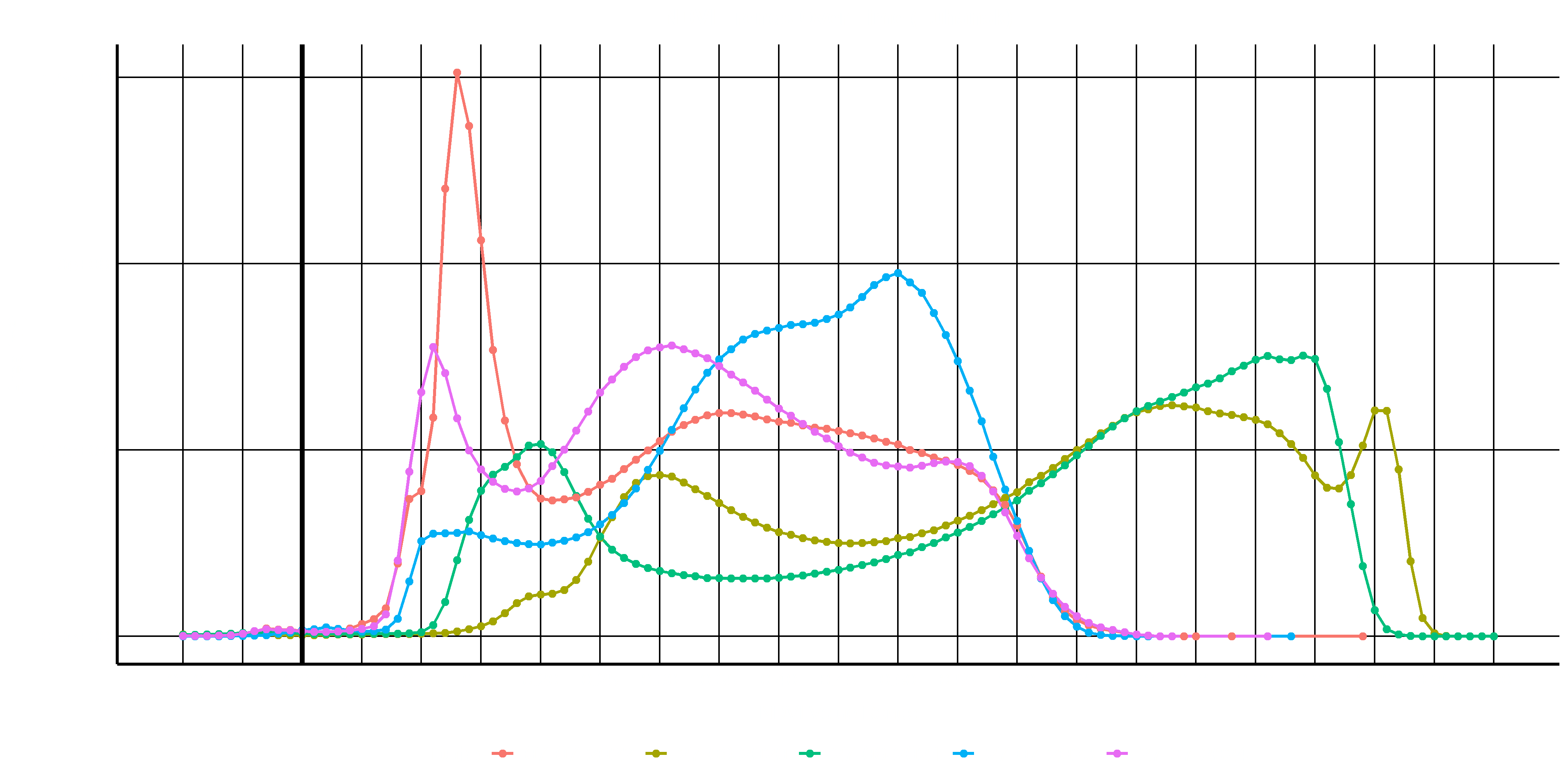
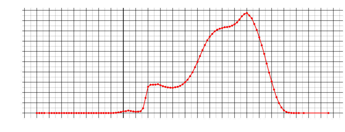
4.2 Visualizing NDVI Data – Bar and Line Plots

This snippet demonstrates how to create custom visualizations for NDVI data using ggplot2. It includes a bar plot and a line plot.

➊

Custom Theme: Defines a consistent theme for plots, setting styles for titles, legends, axis labels, and grid lines.

➋

Bar Plot: Creates a bar plot that visualizes the area (in square meters) for various NDVI ranges across different dates. Key steps include:

Mapping NDVI ranges to the x-axis and area to the y-axis.
Using distinct colors for each date to aid in comparison.
Adding a vertical line at 0 for reference.
Saving the plot to the output directory as a PNG file.

➌

Line Plot: Generates a line plot to show NDVI trends over time. Key features include:

Plotting NDVI ranges on the x-axis and area on the y-axis.
Using a line and points to represent data clearly.
Saving the plot to the output directory as a PNG file.

custom_theme <- theme_minimal() +
    theme(
        legend.position = "bottom",
        legend.box = "horizontal", 
        legend.title = element_text(color = "white", size = 16),
        legend.text = element_text(color = "white", size = 14),
        legend.justification = "center",
        legend.box.spacing = unit(1, 'cm'),
        legend.spacing.x = unit(1.5, 'cm'),
        legend.key = element_rect(fill = "transparent"),
        plot.title = element_text(color = "white", size = 14, face = "bold", hjust = 0.5, margin = margin(b = 10)),
        axis.title.x = element_text(color = "white", size = 12, margin = margin(t = 10)),
        axis.title.y = element_text(color = "white", size = 12, margin = margin(r = 10)),
        axis.text.x = element_text(color = "white", size = 12),
        axis.text.y = element_text(color = "white", size = 12),
        panel.grid.major = element_line(color = "black", size = 0.5),
        panel.grid.minor = element_blank(),
        panel.grid.major.x = element_line(color = "black", size = 0.5),
        panel.grid.major.y = element_line(color = "black", size = 0.5, linetype = "solid"),
        scale_y_continuous(breaks = seq(0, max(all_grouped_data$area_m2, na.rm = TRUE), by = 2.5e+07)),
        axis.line.x = element_line(color = "black", size = 1),
        axis.line.y = element_line(color = "black", size = 1),
        panel.background = element_rect(fill = "transparent", color = NA),
        plot.background = element_rect(fill = "transparent", color = NA)
    )
    theme(
        legend.position = "bottom",
        legend.box = "horizontal",
        legend.title = element_text(color = "white", size = 16),
        legend.text = element_text(color = "white", size = 14),
        legend.spacing.x = unit(20, 'mm'),
        legend.key = element_rect(fill = "transparent"),
        plot.title = element_text(color = "white", size = 14, face = "bold", hjust = 0.5, margin = margin(b = 10)),
        axis.title.x = element_text(color = "white", size = 12, margin = margin(t = 10)),
        axis.title.y = element_text(color = "white", size = 12, margin = margin(r = 10)),
        axis.text.x = element_text(color = "white", size = 12),
        axis.text.y = element_text(color = "white", size = 12),
        panel.grid.major = element_line(color = "black", size = 0.5),
        panel.grid.minor = element_blank(),
        panel.grid.major.x = element_line(color = "black", size = 0.5),
        panel.grid.major.y = element_line(color = "black", size = 0.5),
        axis.line.x = element_line(color = "black", size = 1),
        axis.line.y = element_line(color = "black", size = 1),
        panel.background = element_rect(fill = "transparent", color = NA),
        plot.background = element_rect(fill = "transparent", color = NA)
    )
    theme(legend.key.width = unit(3, 'cm'), legend.spacing.x = unit(2, 'cm')) +
    theme(legend.spacing.x = unit(15, 'mm')) +
    theme(legend.spacing.x = unit(5, 'mm')) +
    theme(
        plot.title = element_text(color = "white", size = 14, face = "bold", hjust = 0.5, margin = margin(b = 10)),
        axis.title.x = element_text(color = "white", size = 12, margin = margin(t = 10)),
        axis.title.y = element_text(color = "white", size = 12, margin = margin(r = 10)),
        axis.text.x = element_text(color = "white", size = 12),
        axis.text.y = element_text(color = "white", size = 12),
        legend.title = element_text(color = "white", size = 16),
        legend.text = element_text(color = "white", size = 14),
        legend.position = "bottom",
        legend.box = "horizontal",
        panel.grid.major = element_line(color = "black", size = 0.5),
        panel.grid.minor = element_blank(),
        panel.grid.major.x = element_line(color = "black", size = 0.5),
        panel.grid.major.y = element_line(color = "black", size = 0.5),
        axis.line.x = element_line(color = "black", size = 1),
        axis.line.y = element_line(color = "black", size = 1),
        panel.background = element_rect(fill = "transparent", color = NA),
        plot.background = element_rect(fill = "transparent", color = NA)
    )

bar_plot <- ggplot(all_grouped_data, aes(x = range, y = area_m2, fill = date)) +
    geom_bar(stat = "identity", position = "dodge") +
    labs(
        title = "NDVI Distribution Over Time (Luhansk)",
        x = "NDVI Value Range",
        y = "Area (m²)",
        fill = "Date"
    ) +
    scale_x_continuous(breaks = seq(-0.1, 1, by = 0.05)) +
    geom_vline(xintercept = 0, color = "black", size = 1.5) +
    custom_theme

bar_plot_path <- file.path(output_directory, "Luhansk_NDVI_Distribution_Compared_Years.png")
ggsave(bar_plot_path, plot = bar_plot, width = 14, height = 7, bg = "transparent")
cat("Bar plot saved to", bar_plot_path, "\n")

line_plot <- ggplot(all_grouped_data, aes(x = range, y = area_m2, color = date, group = date)) +
    geom_line(size = 1) +
    geom_point(size = 2) +
    labs(
        title = "NDVI Trends Over Time (Luhansk)",
        x = "NDVI Value Range",
        y = "Area (m²)",
        color = "Date"
    ) +
    scale_x_continuous(breaks = seq(-0.1, 1, by = 0.05)) +
    geom_vline(xintercept = 0, color = "black", size = 1.5) +
    custom_theme

line_plot_path <- file.path(output_directory, "Luhansk_NDVI_Trends_Over_Years.png")
ggsave(line_plot_path, plot = line_plot, width = 14, height = 7, bg = "transparent")
cat("Line plot saved to", line_plot_path, "\n")

5. Using RStudio to generate separate graphs for each year
A single complete R snippet - black & white version

if (!requireNamespace("dplyr", quietly = TRUE)) {
    install.packages("dplyr")
}
if (!requireNamespace("ggplot2", quietly = TRUE)) {
    install.packages("ggplot2")
}
library(dplyr)
library(ggplot2)

file_paths <- list(
    "C:/GIS/NDVILuhanska20200627.csv",
    "C:/GIS/NDVILuhanska20210627.csv",
    "C:/GIS/NDVILuhanska20220707.csv",
    "C:/GIS/NDVILuhanska20230727.csv",
    "C:/GIS/NDVILuhanska20240727.csv"
)
output_directory <- "C:/GIS"
process_file <- function(file_path, output_directory) {
    file_name <- tools::file_path_sans_ext(basename(file_path))
    date_part <- gsub("NDVILuhanska", "", file_name)
    date_formatted <- paste(substr(date_part, 7, 8), substr(date_part, 5, 6), substr(date_part, 1, 4), sep = "-")
    year_formatted <- substr(date_part, 1, 4)
    ndvi_data <- tryCatch({
        read.csv(file_path, header = FALSE)
    }, error = function(e) {
        stop(paste("Failed to load the CSV file:", file_path))
    })
    
    ndvi_values <- as.vector(as.matrix(ndvi_data))
    ndvi_values <- suppressWarnings(as.numeric(ndvi_values))
    ndvi_values <- ndvi_values[!is.na(ndvi_values)]
    ndvi_values <- cut(ndvi_values, breaks = seq(-1, 1, by = 0.01), include.lowest = TRUE, labels = FALSE)
    
    ndvi_df <- data.frame(
        value = ndvi_values,
        original_value = as.vector(as.matrix(ndvi_data))[seq_along(ndvi_values)],
        scaled_value = scale(as.numeric(ndvi_values)),
        sqrt_value = sqrt(abs(as.numeric(ndvi_values)))
    )
    
    result <- ndvi_df %>%
        group_by(value) %>%
        summarise(
            count = n(),
            area_m2 = count * 100,
            mean_scaled_value = mean(scaled_value, na.rm = TRUE),
            sum_sqrt_value = sum(sqrt_value, na.rm = TRUE)
        )
    
    csv_output_path <- file.path(output_directory, paste0(file_name, "_grouped_values.csv"))
    tryCatch({
        write.csv(result, csv_output_path, row.names = FALSE)
        cat("Results saved to", csv_output_path, "\n")
    }, error = function(e) {
        stop(paste("Failed to save results for:", file_name))
    })
    
    bar_plot <- ggplot(result, aes(x = as.numeric(value) * 0.01 - 1, y = area_m2)) +
        geom_bar(stat = "identity", fill = "black") +
        labs(
            title = paste("", year_formatted),
            x = "Range of NDVI Values",
            y = "Area (m²)"
        ) +
        scale_x_continuous(
            limits = c(-0.1, NA),
            breaks = seq(-1, 1, by = 0.05),
            labels = function(x) ifelse((seq_along(x) - 1) %% 2 == 0, x, "")
        ) +
        scale_y_continuous(breaks = scales::pretty_breaks(n = 10)) +
        theme_minimal() +
        theme(
            plot.title = element_text(color = "black", size = 14, face = "bold", hjust = 0.5, margin = margin(b = 5)),
            axis.title.x = element_text(color = "black", size = 14, margin = margin(t = 5)),
            axis.title.y = element_text(color = "black", size = 14, margin = margin(r = 5)),
            axis.text.x = element_text(color = "black", size = 12),
            axis.text.y = element_text(color = "black", size = 12),
            panel.grid.major = element_line(color = "gray", size = 0.5),
            panel.grid.minor = element_line(color = "gray", size = 0.2),
            panel.background = element_rect(fill = "white", color = NA),
            plot.background = element_rect(fill = "white", color = NA)
        )
    
    bar_plot_path <- file.path(output_directory, paste0(file_name, "_bar_plot.png"))
    tryCatch({
        ggsave(bar_plot_path, plot = bar_plot, width = 13, height = 5, bg = "white")
        cat("Bar plot saved to", bar_plot_path, "\n")
    }, error = function(e) {
        stop(paste("Failed to save bar plot for:", file_name))
    })
    
    line_plot <- ggplot(result, aes(x = as.numeric(value) * 0.01 - 1, y = area_m2)) +
        geom_line(color = "black", size = 1) +
        geom_point(color = "black", size = 2) +
        labs(
            title = paste("", year_formatted),
            x = "Range of NDVI Values",
            y = "Area (m²)"
        ) +
        scale_x_continuous(
            limits = c(-0.1, NA),
            breaks = seq(-1, 1, by = 0.05),
            labels = function(x) ifelse((seq_along(x) - 1) %% 2 == 0, x, "")
        ) +
        scale_y_continuous(breaks = scales::pretty_breaks(n = 10)) +
        theme_minimal() +
        theme(
            plot.title = element_text(color = "black", size = 14, face = "bold", hjust = 0.5, margin = margin(b = 5)),
            axis.title.x = element_text(color = "black", size = 14, margin = margin(t = 5)),
            axis.title.y = element_text(color = "black", size = 14, margin = margin(r = 5)),
            axis.text.x = element_text(color = "black", size = 12),
            axis.text.y = element_text(color = "black", size = 12),
            panel.grid.major = element_line(color = "gray", size = 0.5),
            panel.grid.minor = element_line(color = "gray", size = 0.2),
            panel.background = element_rect(fill = "white", color = NA),
            plot.background = element_rect(fill = "white", color = NA)
        )
    
    line_plot_path <- file.path(output_directory, paste0(file_name, "_line_plot.png"))
    tryCatch({
        ggsave(line_plot_path, plot = line_plot, width = 13, height = 5, bg = "white")
        cat("Line plot saved to", line_plot_path, "\n")
    }, error = function(e) {
        stop(paste("Failed to save line plot for:", file_name))
    })
    cat("Processing completed for:", file_path, "\n")
}

for (file_path in file_paths) {
    process_file(file_path, output_directory)
}

6. Using RStudio to generate graphs comparing plots over the years
A single complete R snippet - black & white version

if (!requireNamespace("dplyr", quietly = TRUE)) {
    install.packages("dplyr")
}
if (!requireNamespace("ggplot2", quietly = TRUE)) {
    install.packages("ggplot2")
}
if (!requireNamespace("readr", quietly = TRUE)) {
    install.packages("readr")
}
library(dplyr)
library(ggplot2)
library(readr)

grouped_file_paths <- list(
    "C:/GIS/NDVILuhanska20200627_grouped_values.csv",
    "C:/GIS/NDVILuhanska20210627_grouped_values.csv",
    "C:/GIS/NDVILuhanska20220707_grouped_values.csv",
    "C:/GIS/NDVILuhanska20230727_grouped_values.csv",
    "C:/GIS/NDVILuhanska20240727_grouped_values.csv"
)


output_directory <- "C:/GIS"

all_grouped_data <- data.frame()

for (file_path in grouped_file_paths) {
    file_name <- tools::file_path_sans_ext(basename(file_path))
    date_part <- gsub("NDVI_", "", file_name)
    date_part <- gsub("_grouped_values", "", date_part)
    date_formatted <- paste(substr(date_part, 7, 8), substr(date_part, 5, 6), substr(date_part, 1, 4), sep = "-")
    year_formatted <- substr(date_part, 5, 8)
    
    grouped_data <- tryCatch({
        read.csv(file_path)
    }, error = function(e) {
        stop(paste("Failed to load the grouped CSV file:", file_path))
    })
    
    grouped_data <- grouped_data %>%
        mutate(date = year_formatted, range = as.numeric(value) * 0.01 - 1)
    
    all_grouped_data <- bind_rows(all_grouped_data, grouped_data)
}

all_grouped_data <- all_grouped_data %>%
    filter(range >= -0.1)

custom_theme <- theme_minimal() +
    theme(
        legend.position = "bottom",
        legend.box = "horizontal", 
        legend.title = element_text(color = "black", size = 16),
        legend.text = element_text(color = "black", size = 14),
        plot.title = element_text(color = "black", size = 18, face = "bold", hjust = 0.5, margin = margin(b = 10)),
        axis.title.x = element_text(color = "black", size = 16, margin = margin(t = 10)),
        axis.title.y = element_text(color = "black", size = 16, margin = margin(r = 10)),
        axis.text.x = element_text(color = "black", size = 14),
        axis.text.y = element_text(color = "black", size = 14),
        panel.grid.major = element_line(color = "gray", size = 0.5),
        panel.grid.minor = element_blank(),
        panel.background = element_rect(fill = "white", color = NA),
        plot.background = element_rect(fill = "white", color = NA)
    )

bar_plot <- ggplot(all_grouped_data, aes(x = range, y = area_m2, fill = date)) +
    geom_bar(stat = "identity", position = "dodge") +
    labs(
        title = "NDVI Distribution Over Time",
        x = "NDVI Value Range",
        y = "Area (m²)",
        fill = "Date"
    ) +
    scale_fill_manual(values = gray.colors(n = length(unique(all_grouped_data$date)), start = 0, end = 0.8)) +
    scale_x_continuous(limits = c(-0.1, NA), breaks = seq(-0.1, 1, by = 0.05)) +
    custom_theme

bar_plot_path <- file.path(output_directory, "NDVI_Distribution_Compared_Years.png")
ggsave(bar_plot_path, plot = bar_plot, width = 14, height = 7, bg = "white")
cat("Bar plot saved to", bar_plot_path, "\n")

line_plot <- ggplot(all_grouped_data, aes(x = range, y = area_m2, color = date, group = date)) +
    geom_line(size = 1) +
    geom_point(size = 2) +
    labs(
        title = "NDVI Trends Over Time",
        x = "NDVI Value Range",
        y = "Area (m²)",
        color = "Date"
    ) +
    scale_color_manual(values = gray.colors(n = length(unique(all_grouped_data$date)), start = 0, end = 0.8)) +
    scale_x_continuous(limits = c(-0.1, NA), breaks = seq(-0.1, 1, by = 0.05)) +
    custom_theme

line_plot_path <- file.path(output_directory, "NDVI_Trends_Over_Years.png")
ggsave(line_plot_path, plot = line_plot, width = 14, height = 7, bg = "white")
cat("Line plot saved to", line_plot_path, "\n")

Warsaw, December 2024

Geographic Analysis with R: GeoTIFF Conversion & NDVI CSV Processing

Geographic Analysis with R: GeoTIFF Conversion & NDVI CSV Processing

1. Introduction - code overview

2. Conversion of GeoTIFF Files to CSV

3. Using RStudio to generate separate graphs for each year

3.1 NDVI Data Import – Processing of CSV Files

3.2 Data Transformation – Preparing NDVI Data for Analysis

3.3 Bar Plot Generation – Visualizing NDVI Data

3.4 Line Plot Generation – NDVI Trends Over Ranges

3.5 Batch Processing Completion – Finalizing Workflow

4. Using RStudio to generate graphs comparing plots over the years

4.1 Setting Up Environment – Checking Packages and Preparing Data

4.2 Visualizing NDVI Data – Bar and Line Plots

5. Using RStudio to generate separate graphs for each yearA single complete R snippet - black & white version

6. Using RStudio to generate graphs comparing plots over the yearsA single complete R snippet - black & white version

Geographic Analysis with R:
GeoTIFF Conversion & NDVI CSV Processing

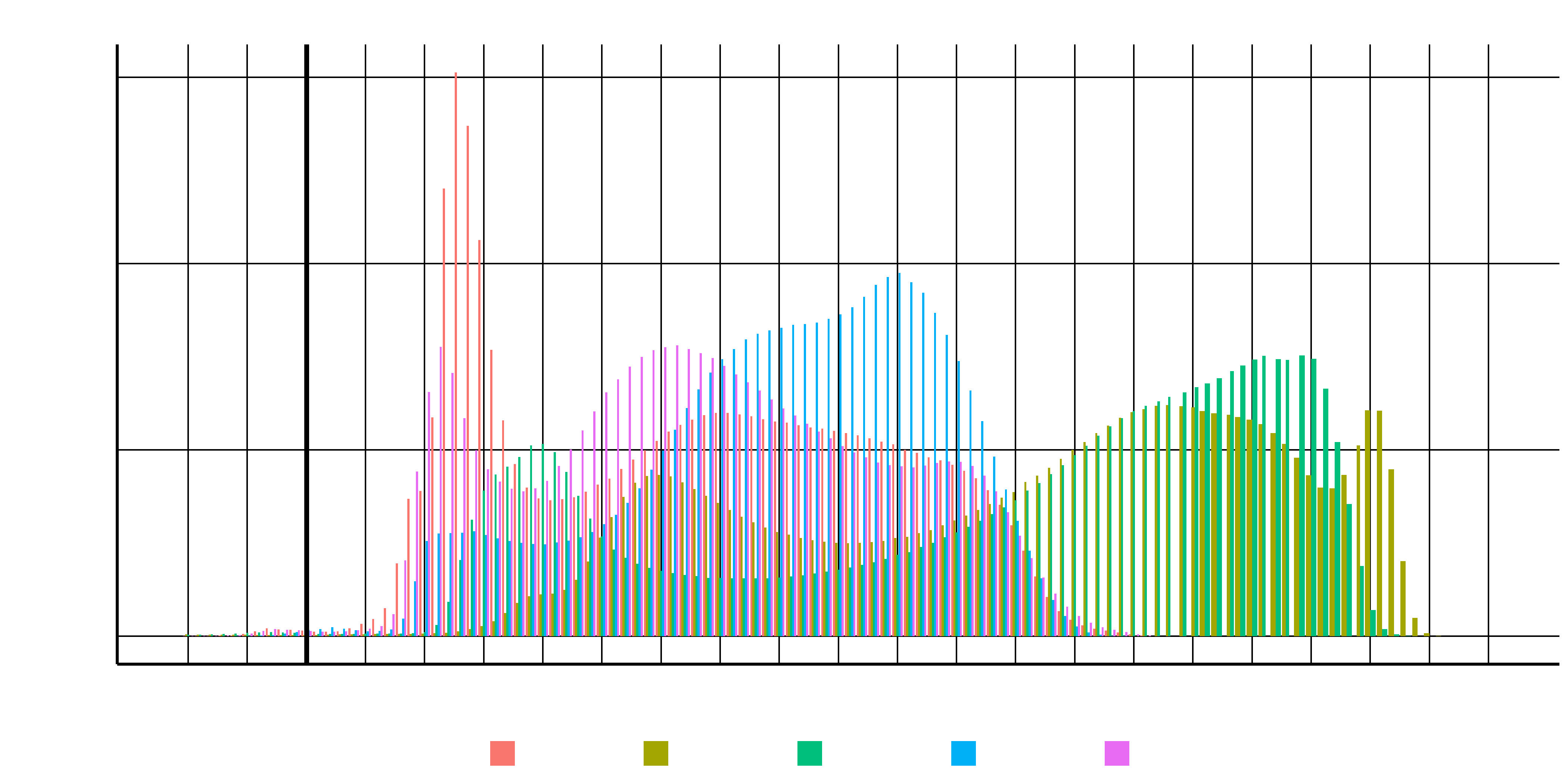
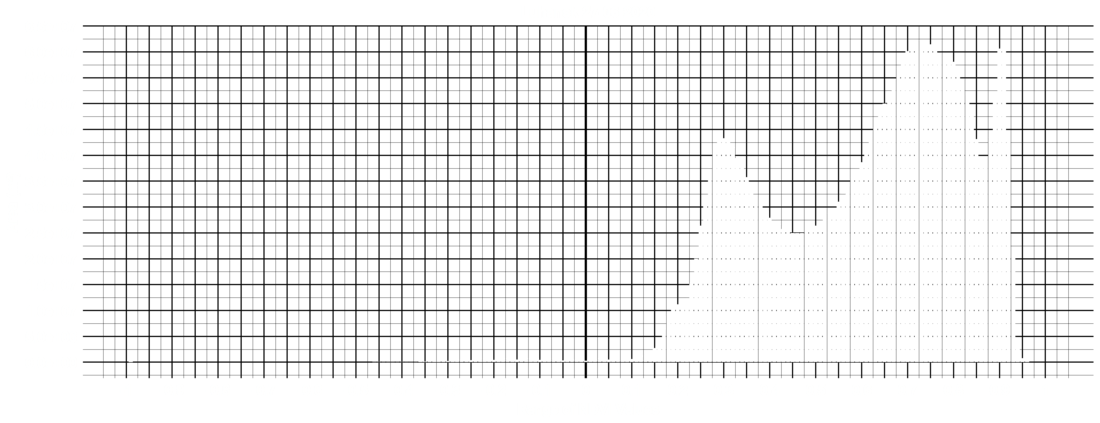
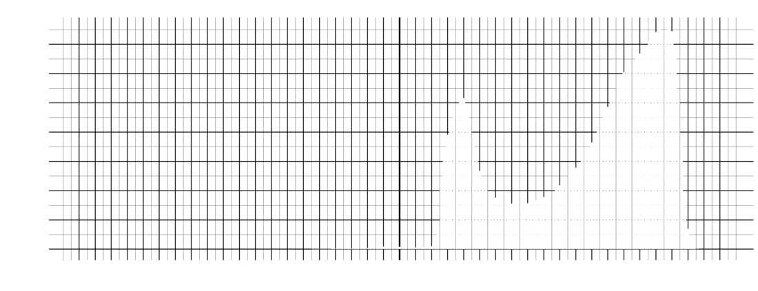
5. Using RStudio to generate separate graphs for each year
A single complete R snippet - black & white version

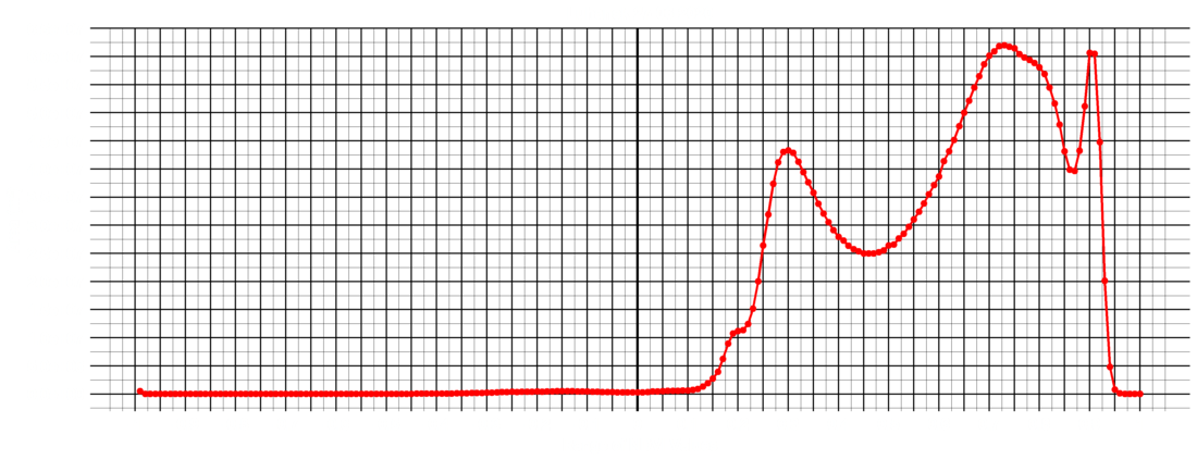
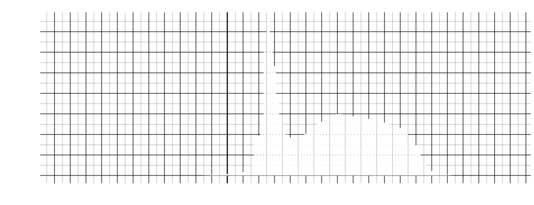
6. Using RStudio to generate graphs comparing plots over the years
A single complete R snippet - black & white version